
Decomposing Softmax for Hardware Acceleration
deep-dive into how softmax can be accelerated in hardware

Softmax is a non-linear function used in the transformer architecture, which powers every LLM. It’s specifically used in the attention mechanism, where we perform:
Unlike feed-forward layers, where the non-linearities are interchangeable (i.e. RELU, sigmoid, softmax), the attention mechanism is strict about using softmax, making it an essential part of the computation. As part of an overarching transformer inference accelerator project I’m working on, I decided to build a custom hardware pipeline for softmax computation.
What is softmax?
Like many other non-linearities, softmax is a function used to normalize a set of values. Given an input vector, softmax applies a transformation on that vector to squeeze all of the values between 0 and 1. Intuitively, it transforms all of the values inside the vector into probabilities, which, when summed, equal to 1. This plays a crucial role in ML, as the goal of any model is to output the highest probability prediction.

Mathematically, the equation is:
Each element is exponentiated, then divided by the sum of all of the exponentiated elements.
Modern ML frameworks like PyTorch and TensorFlow have built in functions for softmax, which can be computed with one simple call. Even if you were to go about building it from scratch in C or Python, it’s relatively straightforward. In hardware, however, the difficulty increases because there are no built-in operators for exponentiation and division.
How can we build this in hardware?
In principle, it’s similar to how we would build softmax in any other programming language - we have blocks of computation (division, exp, accumulate) that we send the data through, in an orderly manner. However, there are some things we have to add and account for in hardware.
In any hardware design, there’s 3 key parameters that will affect your design choices: throughput, latency, and clock speed. In industry, clock speed is constraint given by a client, but for me it’s a non-factor, so the only parameters I’m considering are throughput and latency. Throughput is the amount of data that can be processed in a certain amount of time, where as latency is the amount of time it takes for a given input to be processed as an output. Think of them as the inverse of one another.
The parameter I’m optimizing for is throughput. To do so, I followed a pipelined approach, where I buffered the data using FIFOs. Virtually any buffer could be used to store these values but I chose FIFOs for their simplicity. They follow a first-in-first-out format, where the data exits the memory in the same order as it was written to the memory. It can be visualized as a queue of people waiting for something.
Using buffers allows other inputs to enter the pipeline while previous inputs haven’t fully been processed yet, meaning there’s almost always more than one input being processed in the pipeline, achieving high parallelism.

The data flows as follows:
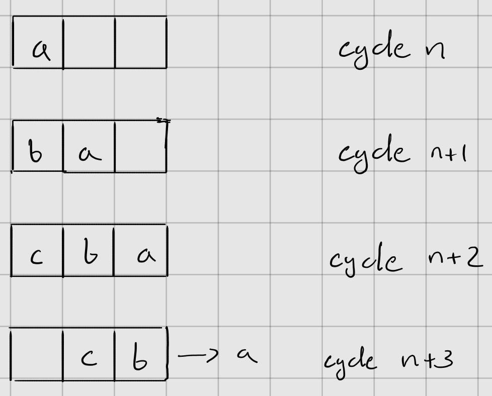
The first input gets stored as the max value and updates by comparing itself to subsequent input values. Each of these values are stored in FIFO A. This process is repeated for each input while the previous inputs progress through the FIFO, which has a length of 32. By the time all inputs are loaded, the FIFO should be full as well.

how data progresses through a FIFO Each element is individually read from FIFO A and has 2 operations (subtracting the max and exponentiation) performed on it before it enters FIFO B. The same data entering FIFO B is accumulated to find the total sum of the exponentiated values, of which the reciprocal is then computed.
Each value is once again individually read from FIFO B and multiplied by the reciprocal of the sum, resulting in a probability, which, when added together with all of the other probabilities in the vector, should equal 1.
Exponentiation
This was easily the most interesting part for me to learn about and implement. Since exponentiation is a non-linear operation, it can’t be computed using basic operators in Verilog. A commonly used method to approximate non-linearities in hardware is to slice up the e^x function and store the x and y values in look-up tables (LUTs), which are a form of storage available on FPGAs that related values to one another. The problem with this approach is that it would take a lot of storage to get high precision approximations. Fortunately, this can be done in more elegant way — we will still have to approximate the function, but what we can do is significantly reduce the domain over which we have to approximate.
I want to walk through this as if I was inventing it from scratch. We’re given a function e^x and we want to shrink the domain want to approximate over, meaning we need to evaluate e^x with the product of some function and e^p, where p exists on a smaller domain than x. If we think about the simplest operations to perform in hardware, bit-shifting (multiplying by a power of 2) is at the top of that list. In binary, each bit to the left represents a successive power of two, which means multiplying a value by 2^n is equivalent to shifting the value’s bits to the left n times.

This means, if possible, we’d want to somehow express e^x as a product of
where z and p are arbitrary values.
Using logarithmic rules, we can express this as
With exponent rules, we can rewrite this as
We decomposed x into z*ln2 + p. Now that p is the range we would have to approximate e^x over, ideally we’d want it to be as small as possible. We can make this happen by setting z equal to
This sets p to 0, which is the ideal value, so we find z then floor the value and calculate p with
where we’d use the previously calculated z value. The reason we do this is because it guarantees p to fall between -ln2 and 0, since z*ln2 would be the largest multiple of ln2 that can fit into x. This shrinks the range we’d have to approximate over to [-ln2, 0].
Putting everything together, we were able to simplify e^x over some arbitrary range into
We were able to simplify e^x and we can now evaluate most of it with bit shifts. However, we still need to approximate e^p. One way to do this would be use tables to store values, but there is a more elegant and inituitive way to do it - using a polynomial. Intuitively, this makes sense, because e^x and a quadratic function both have curved graphs.

If we tweak the constants in the quadratic function, we can change the shape of the parabola to get as close to the shape of the exponential curve as possible over a given interval. More specifically, we want to minimize the vertical distance between the two curves over the interval of [-ln2, 0].
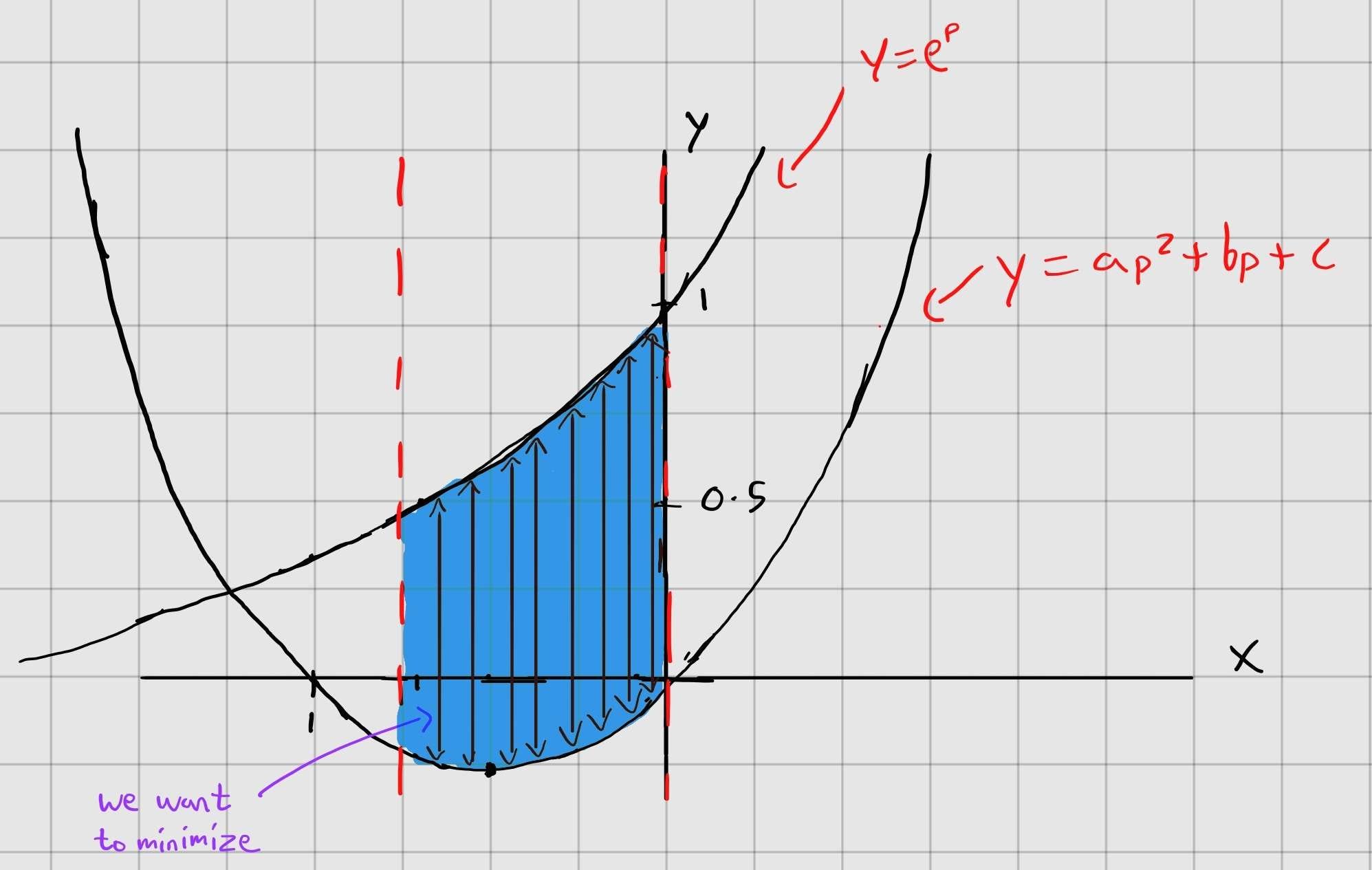
Since we want to minimize the distance between 2 points over an interval, we can represent this as taking the integral of the euclidean distance between these 2 functions over the interval of [-ln2, 0]
where L(p) is the quadratic function ap^2 + bp + c, which can be rewritten as a(p+b)^2 + c. If we expand the integral above, it can be expressed as
Since we want to minimize this integral, we ask “what values of a, b, and c make the integral as small as possible?” To figure this out, we can take the partial derivatives of the integral with respect to each of a, b, and c and set them equal to 0.
This is a system of equations with 3 equations and 3 unknowns, which gives us the values of a, b, and c when we solve it.
So the polynomial approximation of e^p is
and the hardware implementation of e^x is
where z = (x/ln2) and p = x + z*ln2.
It’s a beautiful way of manipulating a function to make it meet certain criteria to be hardware friendly.
Division
Although the “/” operator exists in Verilog and sometimes works in simulation, it doesn’t synthesize into hardware when implemented on an FPGA board. To overcome this, we need to make our own division module. There are a few notable ways to build the division functionality in hardware such as Newton-Raphson division and non-restoring division, but the method I chose to use is restoring division for its simplicity and high parallelism.
This method uses an FSM (finite state machine) and functions as long division in binary. It works as follows:
Remainder R and quotient Q are initialized to 0.
On every cycle, R is shifted left by 1 bit and the i’th bit of the dividend, where i is an index that starts at the bit-width of the values in the divider and is incremented down every clock cycle.
A new value R’ gets stored as R-D.
If R’ >= 0, R becomes R’ and the i’th bit of Q becomes 1. If R’ < 0, R stays the same value and the i’th bit of Q becomes 0.
Once i becomes 0, the value of Q and R are the final quotient and remainder values.
Hopefully it’s somewhat obvious how this is the same as long division in principle, but being performed in base-2. We have a remainder, subtract a multiple of the divisor then update the quotient — although it looks different here because of binary numbers, it’s the same concept.
Next Steps
Implementing those two functionalities and figuring how to buffer the data was 90% of the work with this module. I want to make some changes later to the exponentiation module, as it’s purely combinational right now and I can easily improve throughput by making it pipelined.
My next goal is to finish the overarching project this was a part of — a transformer inference accelerator, with the end goal of testing it with I-BERT (an integer version of an encoder-only LLM). Stick around if you’d like to see it through :)
You can find my code here and the original paper that inspired this post here.